
Data science demonstrates its value when applied to practical challenges. This article shares insights gained from hands-on machine learning projects.
In my experience with machine learning and data science, transitioning from development to production is a critical and challenging phase. This process typically unfolds in iterative steps, gradually refining the product until it meets acceptable standards. Along the way, I’ve observed recurring pitfalls that often slow down the journey to production.
This article explores some of these challenges, focusing on the pre-release process. A separate article will go into depth on the post-production lifecycle of a project in greater detail.
I believe the iterative cycle is integral to the development process, and my goal is to optimize it, not eliminate it. To make the concepts more tangible, I’ll use the Kaggle Fraud Detection dataset (DbCL license) as a case study. For modeling, I’ll leverage TabNet and Optuna for hyperparameter optimization. For a deeper explanation of these tools, please refer to my previous article.
Optimizing Loss Functions and Metrics for Impact
When starting a new project, it’s essential to clearly define the ultimate objective. For example, in fraud detection, the qualitative goal — catching fraudulent transactions — should be translated into quantitative terms that guide the model-building process.
There is a tendency to default to using the F1 metric to measure results and an unweighted cross entropy loss function, BCE loss, for categorical problems. And for good reasons — these are very good, robust choices for measuring and training the model. This approach remains effective even for imbalanced datasets, as demonstrated later in this section.
To illustrate, we’ll establish a baseline model trained with a BCE loss (uniform weights) and evaluated using the F1 score. Here’s the resulting confusion matrix.

The model shows reasonable performance, but it struggles to detect fraudulent transactions, missing 13 cases while flagging only one false positive. From a business standpoint, letting a fraudulent transaction occur may be worse than incorrectly flagging a legitimate one. Adjusting the loss function and evaluation metric to align with business priorities can lead to a more suitable model.
To guide the model choice towards prioritizing certain classes, we adjusted the F-beta metric. Looking into our metric for choosing a model, F-beta, we can make the following derivation.
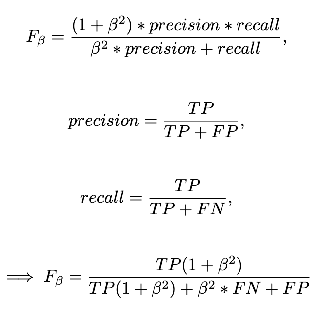
Here, one false positive is weighted as beta square false negatives. Determining the optimal balance between false positives and false negatives is a nuanced process, often tied to qualitative business goals. In an upcoming article, we will go more in depth in how we derive a beta from more qualitative business goals. For demonstration, we’ll use a weighting equivalent to the square root of 200, implying that 200 unnecessary flags are acceptable for each additional fraudulent transaction prevented. Also worth noting, is that as FN and FP goes to zero, the metric goes to one, regardless of the choice of beta.
For our loss function, we have analogously chosen a weight of 0.995 for fraudulent data points and 0.005 for non fraudulent data points.

The results from the updated model on the test set are displayed above. Apart from the base case, our second model prefers 16 cases of false positives over two cases of false negatives. This tradeoff is in line with the nudge we hoped to get.
Prioritize Representative Metrics Over Inflated Ones.
In data science, competing for resources is common, and presenting inflated results can be tempting. While this might secure short-term approval, it often leads to stakeholder frustration and unrealistic expectations.
Instead, presenting metrics that accurately represent the current state of the model fosters better long-term relationships and realistic project planning. Here’s a concrete approach.
Split the data accordingly.
Split the dataset to mirror real-world scenarios as closely as possible. If your data has a temporal aspect, use it to create meaningful splits. I have covered this in a prior article, for those wanting to see more examples.
In the Kaggle dataset, we will assume the data is ordered by time, in the Time column. We will do a train-test-val split, on 80%, 10%, 10%. These sets can be thought of as: You are training with the training dataset, you are optimising parameters with the test dataset, and you are presenting the metrics from the validation dataset.
Note, that in the previous section we looked at the results from the test data, i.e. the one we are using for parameter optimisation. The validation data set which held out, we now will look into.

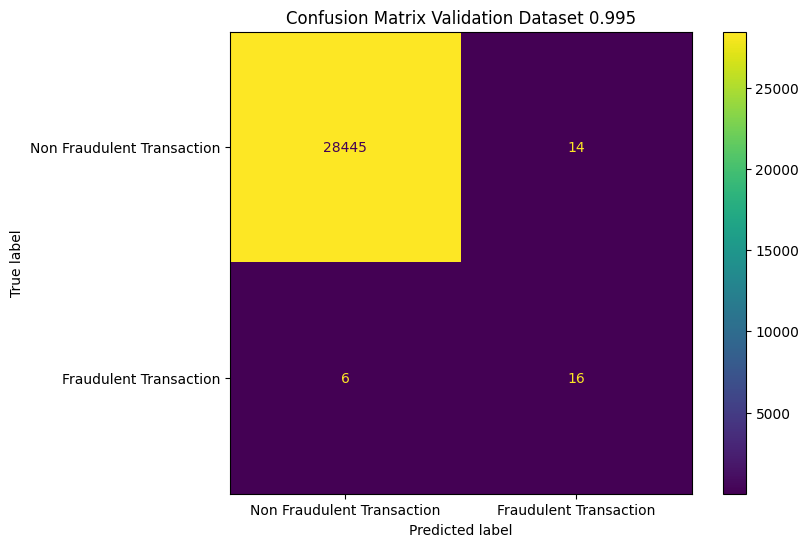
We observe a drop in recall from 75% to 68% and from 79% to 72%, for our baseline and weighted models respectively. This is expected, as the test set is optimized during model picking. The validation set, however, gives a more honest assessment.
Be Mindful of Model Uncertainty.
As in manual decision making, some data points are more difficult than others to assess. And the same phenomena might occur from a modelling perspective. Addressing this uncertainty can facilitate smoother model deployment. For this business purpose — do we have to classify all data points? Do we have to give a pont estimate or is a range sufficient? Initially focus on limited, high-confidence predictions.
These are two possible scenarios, and their solutions respectively.
Classification.
If the task is classification, consider implementing a threshold on your output. This way, only the labels the model feels certain about will be outputted. Else, the model will pass the task, not label the data. I have covered this in depth in this article.
Regression.
The regression equivalent of the thresholding for the classification case, is to introduce a confidence interval rather than presenting a point estimate. The width of the confidence is determined by the business use case, but of course the trade off is between prediction accuracy and prediction certainty. This topic is discussed further in a previous article.
Model Explainability
Incorporating model explainability is to prefer whenever possible. While the concept of explainability is model-agnostic, its implementation can vary depending on the model type.
The importance of model explainability is twofold. First is building trust. Machine learning still faces skepticism in some circles. Transparency helps reduce this skepticism by making the model’s behavior understandable and its decisions justifiable.
The second is to detect overfitting. If the model’s decision-making process doesn’t align with domain knowledge, it could indicate overfitting to noisy training data. Such a model risks poor generalization when exposed to new data in production. Conversely, explainability can provide surprising insights that enhance subject matter expertise.
For our use case, we’ll assess feature importance to gain a clearer understanding of the model’s behavior. Feature importance scores indicate how much individual features contribute, on average, to the model’s predictions.

This is a normalized score across the features of the dataset, indicating how much they are used on average to determine the class label.
Consider the dataset as if it were not anonymized. I have been in projects where analyzing feature importance has provided insights into marketing effectiveness and revealed key predictors for technical systems, such as during predictive maintenance projects. However, the most common reaction from subject matter experts (SMEs) is often a reassuring, “Yes, these values make sense to us.”
An in-depth article exploring various model explanation techniques and their implementations is forthcoming.
Preparing for Data and Label Drift in Production Systems
A common but risky assumption is that the data and label distributions will remain stationary over time. Based on my experience, this assumption rarely holds, except in certain highly controlled technical applications. Data drift — changes in the distribution of features or labels over time — is a natural phenomenon. Instead of resisting it, we should embrace it and incorporate it into our system design.
A few things we might consider is to try to build a model that is better to adapt to the change or we can set up a system for monitoring drift and calculate it’s consequences. And make a plan when and why to retrain the model. An in depth article within drift detection and modelling strategies will be coming up shortly, also covering explanation of data and label drift and including retraining and monitoring strategies.
For our example, we’ll use the Python library Deepchecks to analyze feature drift in the Kaggle dataset. Specifically, we’ll examine the feature with the highest Kolmogorov-Smirnov (KS) score, which indicates the greatest drift. We view the drift between the train and test set.
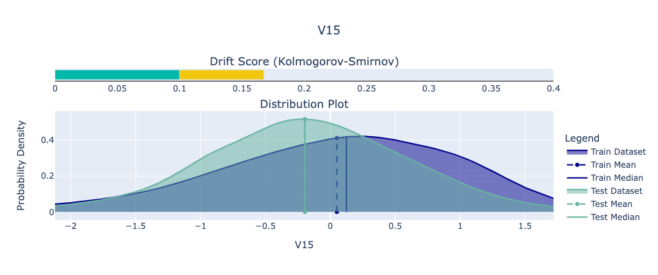
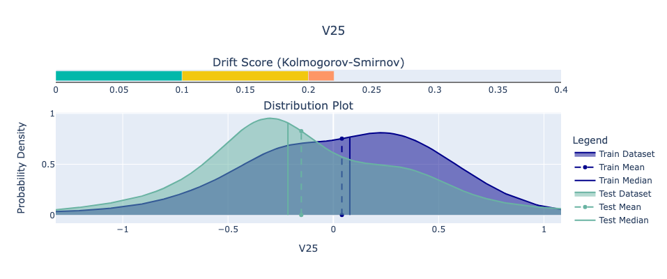
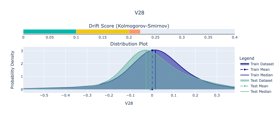
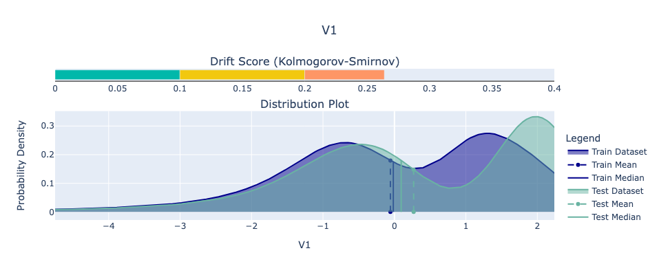
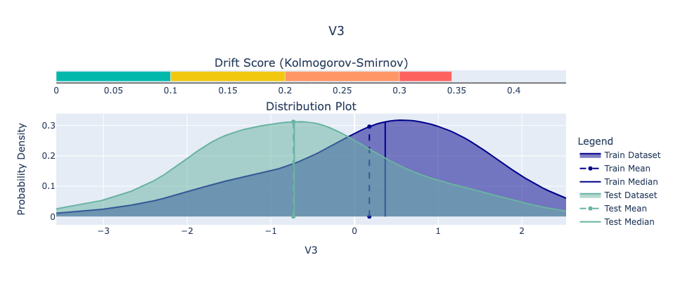
While it’s difficult to predict exactly how data will change in the future, we can be confident that it will. Planning for this inevitability is critical for maintaining robust and reliable machine learning systems.
Summary
Bridging the gap between machine learning development and production is no small feat — it’s an iterative journey full of pitfalls and learning opportunities. This article dives into the critical pre-production phase, focusing on optimizing metrics, handling model uncertainty, and ensuring transparency through explainability. By aligning technical choices with business priorities, we explore strategies like adjusting loss functions, applying confidence thresholds, and monitoring data drift. After all, a model is only as good as its ability to adapt — similar to human adaptability.
Thank you for taking the time to explore this topic.
I hope this article provided valuable insights and inspiration. If you have any comments or questions, please reach out. You can also connect with me on LinkedIn.
Real World Use Cases: Strategies that Will Bridge the Gap Between Development and Productionizing was originally published in Towards Data Science on Medium, where people are continuing the conversation by highlighting and responding to this story.

 Add to favorites


0 Comments